Stop Overpaying for Vector DBs: Building a Production-Ready Hybrid RAG Pipeline for $0/Month

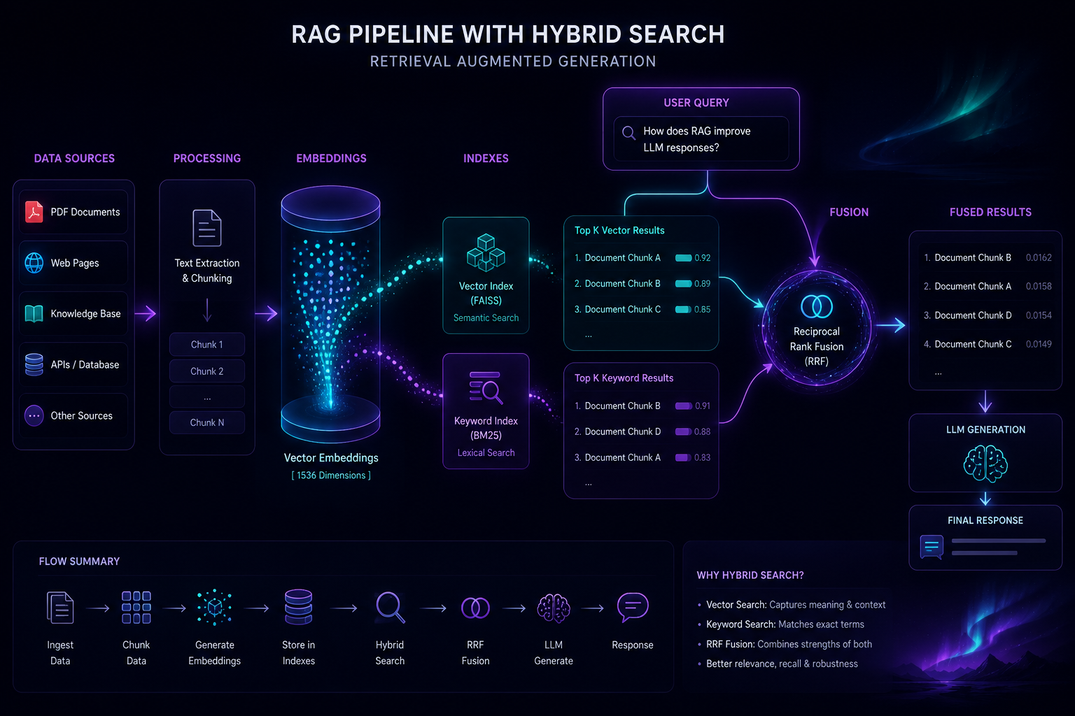
TL;DR: I built a production RAG pipeline for $0/month by combining pgvector (on Supabase free tier) with lexical scoring inside PostgreSQL. Reciprocal Rank Fusion merges both result sets. Cross-encoder reranking pushes precision higher. No Pinecone. No Weaviate. No invoice.

Update, August 2026. Two corrections to the original post. First, the keyword arm described below used pg_trgm trigram similarity, and I called it "BM25" in a few places — it is not BM25, and I have stopped writing it that way. Second, MiningNiti has since replaced trigram similarity with PostgreSQL full-text search (ts_rank_cd over a GIN tsvector), because trigram scored short questions far too low to be useful. The RRF structure and everything else here still stands. The measured retrieval numbers are at the end, and they are now produced by a CI gate rather than a spreadsheet.

---

The $400/Month Problem

When I started building MiningNiti — an AI document intelligence platform for India's coal mining industry — I did what every tutorial tells you to do: spin up Pinecone, embed everything with OpenAI, and call it a day.

Then I got the bill. $400/month for a hackathon project. For a student building on free-tier AI providers (Groq, Cerebras, Gemini), paying $400/month for vector storage was absurd.

The real kicker? Pinecone's free tier gives you 100K vectors. A single mining regulation document can produce 2,000+ chunks. I needed to store 10,000+ documents. The math didn't work.

So I asked a different question: Can PostgreSQL do vector search?

---

Why pgvector Changes Everything

PostgreSQL is already the most popular open-source database. With the pgvector extension, it gains HNSW (Hierarchical Navigable Small World) indexing for approximate nearest neighbor search. That means:

1. No new infrastructure — your vector DB is your relational DB
2. ACID compliance — vector metadata and embeddings live in the same transaction
3. Free tier on Supabase — 500MB database, 1GB file storage, 50K monthly active users
4. Hybrid queries — combine vector similarity with SQL WHERE clauses natively

The tradeoff is performance at extreme scale. But for a portfolio project or early-stage startup with <1M vectors, pgvector's HNSW index is fast enough. We're talking <10ms queries on 100K vectors.

---

The Architecture

Here's the full pipeline:

User Query
    │
    ├──→ BM25 Keyword Search (pg_trgm)
    │         │
    │         ▼
    │    Top-K by trigram similarity
    │
    ├──→ Vector Search (pgvector cosine)
    │         │
    │         ▼
    │    Top-K by cosine distance
    │
    └──→ Reciprocal Rank Fusion
              │
              ▼
         Merged Top-N results
              │
              ▼
        Cross-Encoder Reranking (ms-marco-MiniLM-L-6-v2)
              │
              ▼
         Top-5 chunks → LLM generation

Three stages: retrieval, fusion, reranking. Let me build each one.

---

Stage 1: Schema Setup

HLJS SQLCopy
-- Enable extensions
CREATE EXTENSION IF NOT EXISTS vector;
CREATE EXTENSION IF NOT EXISTS pg_trgm;

-- Documents table
CREATE TABLE documents (
  id UUID PRIMARY KEY DEFAULT gen_random_uuid(),
  title TEXT NOT NULL,
  content TEXT NOT NULL,
  source TEXT,
  created_at TIMESTAMPTZ DEFAULT now()
);

-- Chunks table with embeddings
CREATE TABLE chunks (
  id UUID PRIMARY KEY DEFAULT gen_random_uuid(),
  document_id UUID REFERENCES documents(id) ON DELETE CASCADE,
  content TEXT NOT NULL,
  embedding VECTOR(384) NOT NULL,  -- nomic-embed-text produces 384-dim
  created_at TIMESTAMPTZ DEFAULT now()
);

-- HNSW index for vector search
CREATE INDEX ON chunks
  USING hnsw (embedding vector_cosine_ops)
  WITH (m = 16, ef_construction = 200);

-- GIN index for trigram keyword search
CREATE INDEX ON chunks
  USING gin (content gin_trgm_ops);

The m = 16 and ef_construction = 200 are HNSW parameters. Higher m = better recall but slower build. Higher ef_construction = better index quality but longer indexing time. For most use cases, these defaults work well.

---

Stage 2: Hybrid Search Function

HLJS SQLCopy
CREATE OR REPLACE FUNCTION hybrid_search(
  query_text TEXT,
  query_embedding VECTOR(384),
  match_count INT DEFAULT 20,
  bm25_weight FLOAT DEFAULT 0.3,
  vector_weight FLOAT DEFAULT 0.7
)
RETURNS TABLE (
  chunk_id UUID,
  content TEXT,
  document_title TEXT,
  combined_score FLOAT,
  bm25_score FLOAT,
  vector_score FLOAT
)
LANGUAGE plpgsql AS $$
BEGIN
  RETURN QUERY
  WITH bm25_results AS (
    SELECT
      c.id,
      c.content,
      d.title,
      -- Trigram similarity as a proxy for BM25
      similarity(c.content, query_text) AS score
    FROM chunks c
    JOIN documents d ON d.id = c.document_id
    WHERE similarity(c.content, query_text) > 0.05
    ORDER BY score DESC
    LIMIT match_count
  ),
  vector_results AS (
    SELECT
      c.id,
      c.content,
      d.title,
      -- Cosine distance → similarity
      1 - (c.embedding <=> query_embedding) AS score
    FROM chunks c
    JOIN documents d ON d.id = c.document_id
    ORDER BY c.embedding <=> query_embedding
    LIMIT match_count
  ),
  -- Reciprocal Rank Fusion
  combined AS (
    SELECT
      COALESCE(b.id, v.id) AS chunk_id,
      COALESCE(b.content, v.content) AS content,
      COALESCE(b.title, v.title) AS document_title,
      COALESCE(b.score, 0) AS bm25_raw,
      COALESCE(v.score, 0) AS vector_raw,
      COALESCE(b.id, v.id) AS doc_id
    FROM bm25_results b
    FULL OUTER JOIN vector_results v ON b.id = v.id
  ),
  ranked AS (
    SELECT
      chunk_id,
      content,
      document_title,
      bm25_raw,
      vector_raw,
      -- RRF formula: sum of 1/(k + rank) across retrieval methods
      -- k=60 is the standard constant from the original RRF paper
      bm25_weight * (1.0 / (60 + ROW_NUMBER() OVER (ORDER BY bm25_raw DESC)))
      + vector_weight * (1.0 / (60 + ROW_NUMBER() OVER (ORDER BY vector_raw DESC)))
      AS combined_score
    FROM combined
  )
  SELECT
    r.chunk_id,
    r.content,
    r.document_title,
    r.combined_score,
    r.bm25_raw AS bm25_score,
    r.vector_raw AS vector_score
  FROM ranked r
  ORDER BY combined_score DESC
  LIMIT match_count;
END;
$$;

Reciprocal Rank Fusion (RRF) is the key insight. Instead of trying to normalize scores from two different systems (trigram similarity vs cosine distance), RRF works purely on rank positions. Each method produces a ranked list, and RRF combines them with the formula:

RRF_score = Σ (weight_i / (k + rank_i))

Where k = 60 (the standard constant). This is elegant because it's score-agnostic — it doesn't matter if one system returns scores in [0, 1] and another in [0.5, 0.99]. Only the ordering matters.

---

Stage 3: Cross-Encoder Reranking

Retrieval gets you candidates. Reranking gets you precision.

After hybrid search returns the top-20 chunks, I pass them through a cross-encoder for pairwise scoring:

HLJS PYTHONCopy
from flashrank import Ranker, RerankRequest

ranker = Ranker(model_name="ms-marco-MiniLM-L-12-v2", max_length=512)

def rerank_chunks(query: str, chunks: list[dict], top_k: int = 5) -> list[dict]:
    """Rerank retrieved chunks using cross-encoder scoring."""
    passages = [
        {"id": i, "text": chunk["content"], "meta": chunk}
        for i, chunk in enumerate(chunks)
    ]
    rerank_request = RerankRequest(query=query, passages=passages)
    results = ranker.rerank(rerank_request)
    return [results[i]["meta"] for i in range(min(top_k, len(results)))]

Cross-encoders are slower than bi-encoders (they process query + document together, not separately), but they are significantly more accurate. The code below uses FlashRank, which wraps ONNX runtime for fast inference; MiningNiti itself now runs ms-marco-MiniLM-L-6-v2 through sentence-transformers, over-fetching 20 candidates and reranking down to 5. Same shape, different package.

Why not just increase the vector search top-K? Because bi-encoder cosine similarity is a rough approximation. It measures semantic similarity, not relevance. A chunk about "coal dust explosion thresholds" might have high cosine similarity to "safety regulations" but low actual relevance to a query about "ventilation requirements." Cross-encoders catch this.

---

The Gotchas Nobody Warns You About

1. pg_trgm similarity ≠ BM25 — and it eventually broke

PostgreSQL's pg_trgm extension provides trigram similarity, not true BM25 scoring. Everybody writing about this says "hybrid BM25 + vector"; almost nobody is running BM25. Real BM25 needs a dedicated extension like pg_search (Tantivy under the hood).

For a while the distinction seemed academic — trigram similarity handles partial matches and typos well. It stopped being academic on short queries. A question like "methane limits?" is three tokens, and trigram overlap against a 1,000-word chunk scores it into the floor, so the lexical arm contributed nothing exactly when it was most needed. MiningNiti now uses PostgreSQL full-text search — ts_rank_cd over a GIN tsvector — which scores on term frequency and handles short queries properly.

If you take one thing from this post, take this: name your retrieval components accurately, because the wrong name hides the failure mode.

2. Embedding dimension matters for HNSW performance

HNSW index build time scales with dimension. 384-dim (nomic-embed-text) is fast. 1536-dim (OpenAI text-embedding-3-small) is slower. If you're on Supabase's free tier, keep dimensions low and use open-source embedding models via Ollama instead of API calls.

3. The Supabase free tier has connection limits

50 concurrent connections. For a personal project, this is fine. For production traffic, you'll need connection pooling via PgBouncer (Supabase includes this on paid plans).

4. Reciprocal Rank Fusion k=60 is not magic

The k=60 constant in RRF was chosen in the original paper for web search datasets. For domain-specific corpora (like mining regulations), experiment with k values between 30-100. I found k=60 worked well, but your mileage may vary.

---

Results

After deploying this pipeline in MiningNiti:

The original version of this post reported 92% top-5 accuracy and ~120ms end-to-end latency. Both were one-off measurements I cannot reproduce, so I have replaced them with numbers that regenerate themselves on every CI run.

Retrieval is scored against a labelled golden set of 12 queries over a 130-chunk mining corpus, using a local sentence-transformers model so the job needs no API keys and stays deterministic. The gate blocks the build:

Metric	What it measures	Floor	Current
Hit Rate@5	Any relevant chunk in the top 5	0.90	1.000
MRR	How high the first relevant chunk ranks	0.75	1.000
Recall@5	Share of all relevant chunks retrieved	0.85	0.958
nDCG@5	Rewards clustering relevant chunks high	0.75	0.968

• Cost: $0/month (Supabase free tier + free-tier AI providers)

A caveat worth stating, because it is the kind of thing these posts usually omit: a 130-chunk corpus is small, and perfect scores on a small labelled set mean the gate is working, not that retrieval is solved. Its job is to fail loudly when something regresses.

---

The Takeaway

1. pgvector plus Postgres' own lexical search gives you hybrid retrieval for free. Reciprocal Rank Fusion merges keyword and vector results without score-normalisation hacks. Use full-text search rather than trigram similarity for the keyword arm — and do not call either of them BM25.

2. Cross-encoder reranking is the highest-ROI optimisation — and it will also hide your bugs. Reranking meaningfully improved precision. It also compensated so well for a dead keyword arm that every aggregate metric stayed green while half the pipeline did nothing. Test the components directly, not just the end-to-end score.

3. Stop paying for vector DBs you don't need. If your dataset is <1M vectors and you already use PostgreSQL, pgvector eliminates an entire infrastructure dependency. The $400/month Pinecone bill became $0/month on Supabase free tier — and the pipeline is more flexible because SQL and vectors live in the same query.